Live interactive demos · fly connectome → neural net

Breathing life into AI with the brain's own wiring

Take a slice of real wiring from a fruit fly's brain - mapped connection by connection - and use it as the scaffold for a neural network. It beats a size-matched random network only at what that brain region evolved to do. Pick a region, pick a task, and watch it happen.

3 circuits
navigation · memory · vision, each wired from a real connectome
+7.8-12%
connectome's edge over matched-random, on its native task
0.995
MQAR recall - a fly memory circuit, near the attention ceiling

Aarav Sinha · Scott Harris · Viktor Toth · Alexis Pomares · Phillip Shiu  ·  Eon Systems PBC  ·  July 2026

scroll

A connectome is an inductive bias you can measure

Evolution spent hundreds of millions of years wiring circuits that solve hard problems with tiny nervous systems. We convert those wiring diagrams directly into recurrent networks - one neuron per unit, one synapse per allowed connection - and ask a sharp question the field had skipped: does the specific biological wiring beat a random wiring of the same size, in the same model, on the same task?

From wiring diagram to network

Each biological neuron becomes one recurrent unit; each directed synapse becomes an allowed connection in Wrec. The state evolves as a recurrent update - the connectome is the substrate; only the input, output and (sometimes) the edge weights are trained.

The one control everyone needs

Every connectome result is matched against a network with the same neurons, same edge count, same optimizer, same everything - only the wiring is randomized. That isolates the biology from recurrence, density and parameter count.

random sparse degree-preserving weight-shuffle no-recurrence
The result in one line. The connectome wins its native task by many sigma, and merely ties - or slightly trails - everywhere else. That double dissociation is the evidence that structure carries task-specific computation, not a lucky initialization.
Central complex

Navigation & path integration

A recurrent ring that holds "which way am I facing" and integrates self-motion into a home vector.

+7.8%vs random on path integration · wins frozen & trainable
Mushroom body

Associative memory

Sparse Kenyon-cell coding binds a stimulus to a value and recalls it later without interference.

0.995MQAR recall - near attention's ceiling of 1.00
Optic lobe

Visual motion & optic flow

Layered motion detectors turn a swarm of moving pixels into a clean estimate of self-motion.

+12%vs random on optic flow, in the data-scarce regime

Pick a region, pick a task — watch the wiring win or fail

This is the whole thesis in one control. Choose a brain region, choose a task, and run the head-to-head: the connectome versus a size-matched random network. The bars and the verdict are the real logged results. The advantage lights up green on the native diagonal and goes flat or red everywhere else.

Brain region
Task

real logged data Numbers are read from the project's result files; every cell reports the real connectome-vs-random advantage and raw scores from the project's result files (published as Figure 1).

The fly's compass - where the computation is the wiring

The central complex is a ring of neurons where a single bump of activity marks heading, sweeping around the ring as the fly turns. Take the controls below: steer a fly, watch the bump rotate and a home vector accumulate - then scramble the wiring and watch the compass drift.

illustrative sandboxreal benchmark belowsee the data
Path-integration sandbox
Two integrators, same size

Hold ← → to turn, to walk (or drag on the arena). Both a connectome ring and a random ring track your heading - watch their estimates of "home" drift apart.

Connectome error
0.00
Random error
0.00
Heading ringThe bump = the network's current heading estimate
Home erroraccumulated heading error (rad) over the walk

We froze the connectome's recurrent circuit and let only its inputs and outputs learn, so any advantage has to come from the wiring itself. On path integration - the exact job this circuit evolved to do - the real connectome tracked heading to about 1.09° and beat every degree-matched control, with all six rewirings strictly worse and zero overlap. Shuffling connections while keeping each neuron's partner-count destroys the gain, pinning the advantage on topology, not cell counts.

A ring attractor is a compact, remarkably stable way to hold and update a continuous variable. Because the useful structure survives freezing, it can be dropped into a larger model as a fixed prior - pointing toward drift-free dead-reckoning for drones and robots in GPS-denied settings.

Heading error vs sequence length (rad, lower = better)

Hemibrain CX · 7,349 neurons / ~512k edges · 3 seeds. The connectome has the lowest error at every length; weight-shuffle tracks it (topology), while no-recurrence collapses.

A memory wired like a fly - near attention, at a fraction of the machinery

The mushroom body learns "this smell meant food, that one meant a shock." Feed the network stimulus→value pairs, then quiz it. A network wired like a real fly recalls faster and clings to old memories more stubbornly than a same-sized random tangle.

illustrative recall demoreal benchmarks + curvessee the data
Associative memory

Bind each key to a value, then click a key to query. Both models must return the value they were shown. The connectome peaks sharply on the right answer; the random control is fuzzier and sometimes wrong.

Click a key to query it.
Recall confidence over the vocabulary
Connectome Random sparse

Benchmark: MQAR test recall (higher = better)

On the standard associative-recall benchmark used to explain the attention-vs-recurrent gap, the full mushroom body (14,025 neurons) reaches 0.995 - essentially the attention ceiling - and beats size-matched random by ~9 points. Shuffling the weights barely dents it; randomizing which neurons connect erases it. The advantage is the topology.

Honest caveat. Much of this reads as generic structured-recurrence capacity: an optic-lobe connectome truncated to the same size ties the mushroom body. What's cleanly isolated is that biological wiring helps associative memory - not that this one circuit is uniquely gifted.

An odor is paired with reward. Midway, the rule flips - the same odor now signals punishment. A good associative memory must update the association, not just memorize the first label. Press play and watch the connectome re-learn the reversal.

Connectome reversal recall
0.992
Random reversal recall
0.973
Reversal episode · recall over time
Both models learn the odor's value, then the rule flips (red line): recall crashes, then re-learns. The connectome recovers fast and high (0.995 reversal recall); random dips deeper and lags (0.979). It also gets there ~3× faster to begin with (validation loss solved by epoch 17 vs 53).

Learn five odor→valence tasks in sequence, with no replay. Every model learns each task perfectly at first - the question is how much it forgets as new tasks pile on. A frozen connectome holds a stable, low-interference representation that a random matrix can't.

The connectome's value here is as a frozen, forgetting-resistant prior on its native modality - close to the inductive bias continual-learning and on-device systems need to absorb new data without retraining from scratch.
Retention across the task sequence
Final accuracy after all 5 tasks: connectome 0.819 vs random 0.748 (forgetting 0.223 vs 0.308, ~10σ over 3 seeds). All three learn each task equally well - the entire gap is retention.

Nature's motion detector - a head start when data is scarce

The optic lobe turns a swarm of moving pixels into a clean sense of which way the world is sliding past. Steer the scene over a fly-like hex sensor and watch the network read out self-motion - then throttle the training data and watch the connectome's advantage appear exactly where it matters.

illustrative sandboxreal data-efficiency curvesee the data
Optic-flow sandbox
Ego-motion readout

Drag across the sensor (or auto-drift). Local motion on the hex lattice is pooled into an estimate of yaw and translation. The connectome reads it more accurately than a random twin - most of all when it has seen little data.

Training data100%

Slide down to starve both models of training examples.

Connectome RMSE
0.132
Random RMSE
0.143
Live motion - idle -

Data-efficiency curve (RMSE, lower = better)

Connectome Random control

Every comparison pits the connectome against a random network of identical size and sparsity, so any edge comes from the wiring pattern itself. In the biologically realistic sparse regime the fly's motion circuit wins (0.1317 vs 0.1425 RMSE), and the pruned connectome beats its random control at every data budget.

Honest caveat. This is an advantage in data efficiency, not a higher ceiling. Give a large dense trainable matrix enough data and it ties the connectome (0.1251 vs 0.1254) - flip to the Dense tab to see the gap close.

The same task runs on real DSEC event-camera footage shot from moving cars - the low-power, tight-compute corner where a sparse structural prior pays off most.

Real wiring beats random - but only at the job it evolved for

Three brain regions × five tasks. Each cell is the connectome's advantage over a matched-random control. Watch the diagonal light up - each region wins on the one task its circuit evolved to do - while the off-diagonal stays dark. That is a double dissociation.

real logged advantagessee the data

Hover or tap any cell to read what it means. The gold-ringed cells are each region's native task.

The comparison is deliberately brutal: every real connectome is pitted against random networks matched on size, density and degree distribution, so the ~8-12% edge along the diagonal can only come from the specific pattern of connections. A diagonal that lights up while off-diagonal cells stay flat is the cleanest evidence that wiring carries task-specific computation rather than a generic boost.
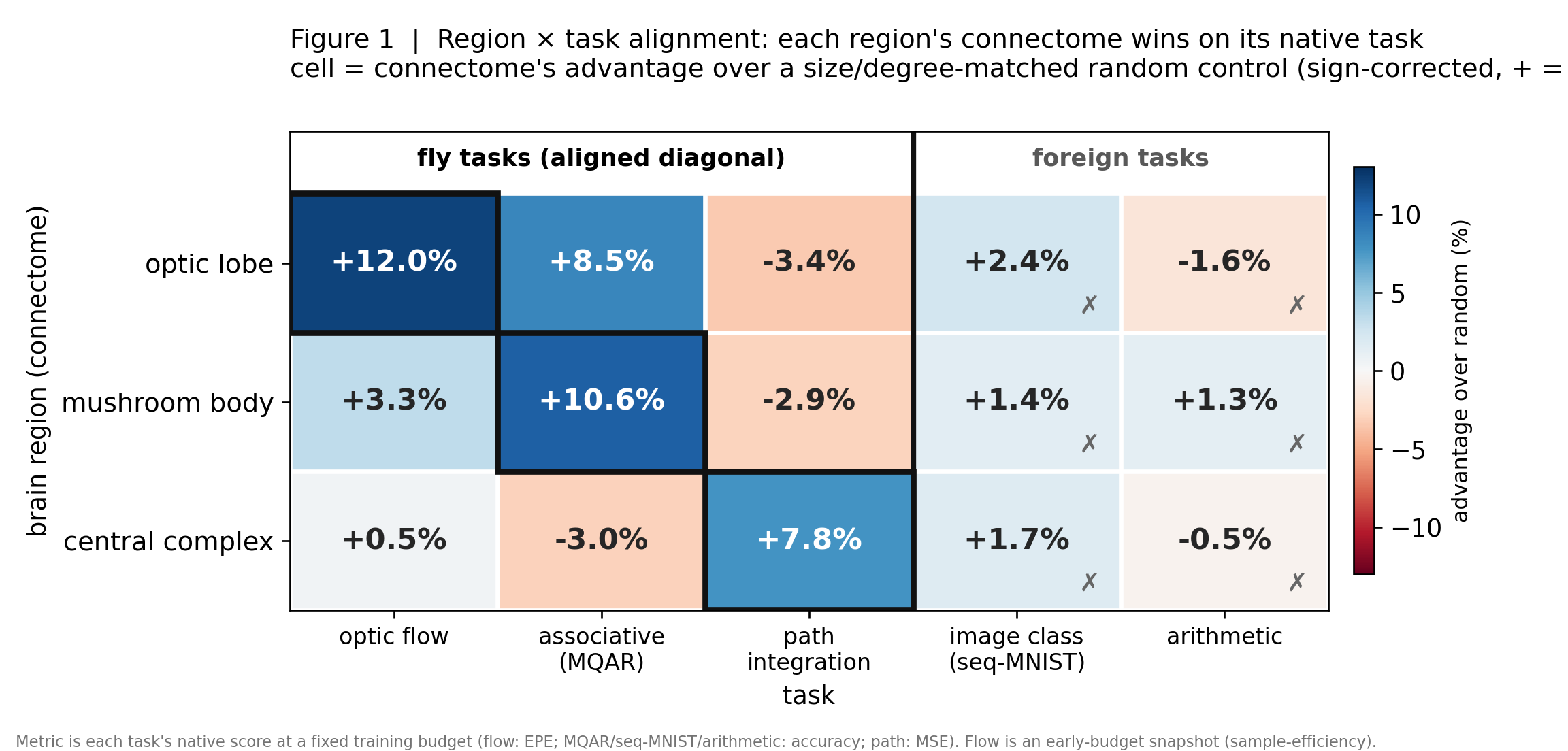
Kept in view. The memory task rewards raw capacity as much as mushroom-body recall, and harder sequential problems (seq-MNIST, arithmetic) stay null for every region. This is a real, bounded signal - not a universal law.
Published region × task alignment matrix
The published Figure 1 - the full alignment matrix from the paper.

Wire the senses in at random - and training routes them back to biology

We never tell the network where the fly's senses plug in. Input arrives smeared at random across all ~11,000 neurons. Yet as it learns the task, the input wiring migrates onto the precise projection neurons the real fly uses. Nobody pointed it there.

illustrative animation of a real resultsee the data

Do input ports find the biological cells?

Connectome Random wiring chance (0.5)
ROC-AUC = how well the learned input weights single out the true biological input cells.

This is emergence you can measure: the input weights' ability to single out the true biological cells climbs from chance (AUC ≈ 0.5) to ≈ 0.6 during training, while a matched random-wired network never leaves chance (p = 3.6 × 10⁻⁵). Because the wiring is the only thing that differs, the pull toward biology has to come from the connectome's structure.

In a model whose recurrent core is a real brain, you can read off which neurons carry which signal after training - turning an opaque network into an inspectable one. A concrete handle on interpretability.
Honest caveat. The effect is real but modest (AUC ≈ 0.6, not 0.9), and it shows up only when the circuit is trained on the task it evolved to do.

The honest science - tightening the test, not selling it

The closest prior work reported that wiring an AI's hidden layer like a fly's brain classifies images better. We reproduced it, added the one control it left out, and the special advantage on generic tasks disappeared. This sharpened the hypothesis instead of inflating it.

real reproduction numberssee the analysis

Add the matched-random control → the edge vanishes

The original comparison changed two things at once - connectome-vs-random and recurrent-vs-feedforward - so its edge on CIFAR-10 couldn't be credited to the wiring alone. Put a random matrix in the exact same architecture and the connectome's advantage on generic image classification evaporates: a matched random-sparse network in fact edges it on both MNIST (0.967 vs 0.965) and CIFAR-10 (0.491 vs 0.468), and a dense trainable matrix beats them all. MNIST still reproduces cleanly (~97%); the underlying work is real. The lesson: a connectome helps only when the task matches the computation its circuitry evolved to perform.

MNIST: connectome 0.965 vs random 0.967 CIFAR-10: connectome 0.468 vs random 0.491 random edges the connectome on both

Same architecture, connectome vs random

Real reproduction numbers. On generic image classification the connectome does not win - random sparse matches or edges it, and dense trainable leads. The special ingredient lives in the architecture around the matrix, not the fly's specific wiring.

The control hierarchy - how we know it's really the topology

connectome ≈ weight-shuffle

Keep the exact wiring, permute the weights, and the win survives → the graph carries it, not the synaptic strengths.

≫ random & degree

Break the wiring - even keeping each neuron's degree - and it falls 9-16 points on MQAR.

no-recurrence → chance

Zero the recurrent path and it collapses (~0.12 on seq-MNIST), proving the recurrence is load-bearing.

frozen vs trainable

Trainable helps the CX (tune one attractor); frozen helps MB continual (protect memories). The verdict tracks the task, not the region.

Limitations & how to read this page
  • Interactive sandboxes are simulations. The fly you steer, the hex sensor, and the recall demo are faithful reproductions of the reported dynamics, not live models. Every chart, bar, and curve is real logged data from the result files (see each "see the data" link).
  • The associative-memory win is partly generic. On MQAR an optic-lobe connectome truncated to the same size ties the mushroom body, so what is cleanly isolated is that biological wiring helps associative recall, not that this one circuit is uniquely gifted.
  • Optic flow is data-efficiency, not a ceiling. The connectome's edge is largest when data is scarce and shrinks as random catches up; a large dense trainable matrix ties it at convergence.
  • The advantage is topological, and small in absolute terms. Weight-shuffle (same wiring, permuted weights) usually tracks the connectome; the CX margins are a few hundredths of a radian, from a single connectome graph (pseudo-replication).
  • Foreign tasks are null. On sequential MNIST and arithmetic the connectome merely ties its topology-matched control. This is a task-specific prior, not a universal architecture.
  • On generic image classification the connectome does not win once the matched-random control is added — it slightly trails random sparse on both MNIST and CIFAR-10 (chart above).

Don't hand-design every module - inherit the circuits evolution already tuned

The fly is the smallest complete brain we can map. As wiring diagrams sharpen - mouse and monkey are arriving now, human is on the horizon - the same three circuits reappear at larger scale, each a candidate prior for the job it evolved to do. Drag through the scale.

Fly

Navigation core

A ring-attractor heading system for drones and edge robots that must localize and hold a course under a tight power budget, in GPS-denied settings - drift-free dead reckoning over long trajectories.

central complex → SLAM · odometry

Event-vision front end

A sparse optic-flow prior for event-camera perception in autonomous vehicles and robots - fast, low-power motion estimation exactly where labeled data and energy are the binding constraints.

optic lobe → DSEC · collision avoidance

Associative memory layer

A forgetting-resistant recall module for chemical & hazard sensors and continual, on-device learning - updating from a handful of noisy labels without retraining from scratch.

mushroom body → few-shot · in-context

A library of evolved, task-specialized priors you compose and fine-tune - instead of hand-designing every module from scratch.

Whether this composes all the way to general intelligence is genuinely open. What is already defensible: mining evolved circuits can beat matched-random baselines on the tasks those circuits were built to solve - aimed squarely at the embodied, data-limited, low-power, continually-changing settings where today's large models are brittle or wasteful.